

Documentation
Notes: here are described mainly technical details about the program. Although I used the premise that the Reader has the specialized knowledge, I have nevertheless tried to formulate things in a more comprehensible form in several places.
Table of contents
From the very first minute of development, the most fundamental aspect was that the application should be useable by anyone, for free, without any registration.
Calculations of phase equilibria are typically complicated, and need a variety of data. So the second aspect became that the program should ask only the absolutely necessary data from the user. It should be as easy-to-use as possible, so the user can focus on the essence of the task. There should be no need for bothering about data that are necessary for the calculations but not interesting for the user.
Therefore, the program was maked very self-propelled. Lots of data were collected, and the app selects what is necessary for the actual task - be it drawing, process modeling, or whatever. A wide variety of materials and their combinations can be applied for a range of issues - whether in education or in industrial practice.
Another aspect of development was reliability. The data of the substances were collected from several sources, as far as possible, in order to eliminate erroneous data. Methods of calculations provide results with the accuracy expected by current professional needs. The application is useful for demonstrational or industrial uses, even though it is not perfect, and there is still room for further improvement.
This application deals basically only with the equilibrium and transition between the vapor and the liquid state, not the solid state. The reason of this is that the non-ideality models used here are not (fully) suitable for handling the solid state. Additionally, solid state addition compounds give much more complicated phase diagrams, than liquid miscibility diagrams or the vapor-liquid equilibrium curves. (In fact, the solid phase adducts cannot be predicted by the methods used by VLE - Calc .com.) Therefore solid-liquid equilibrium (SLE as solubility) became an another project. (Its development is currently suspended).
At the same time, liquid-liquid equilibrium (LLE) and vapor-liquid equilibrium (VLE) are handled together, which has also an important reason, that the model works well only used them together (VLLE). In case of multicomponent systems, before doing any VLE calculation, the program tests the system for liquid stability (is there phase split or not), and if the liquid splits to multiple phases, the program determines the accurate liquid compositions, and only then begins to calculate VLE.
These VLLE calculations are currently used for two purposes: drawing various phase diagrams and modeling distillation.
Approximately 300 compounds can be found in the database, with their identifyers, synonymous names, formulas, basic physical properties, and UNIFAC functional groups describing the structures. The data were taken from several reference sources, in order to eliminate erroneous data.
The physical properties:
- molecular weight (g/mol)
- liquid density (g/cm3)
- melting point (░C)
- boiling point (░C) at 1 atm.
- critical temperature (K)
- critical pressure (bar)
- critical volume (cm3/mol)
- heat capacity of liquid (J/mol*K)
- heat capacity of solid (J/mol*K)
- heat of vaporization (kJ/mol) *
- heat of fusion (kJ/mol)
- heat of sublimation (kJ/mol)
- Antoine constants
- Acentric factor
- Matias-Copeman parameters
*
For some substances either Antoine constans, nor heat of vaporization data could be found in the literature.
But when the normal boiling point and a vapor pressure data at another temperature
(generally room temperature) were available, the heat of vaporization were
calculated from these data using the Clausius-Clapeyron equation (see
chapter 4.1).
Vapor pressure of a pure substance is calculated usually with the Antoine-formula, which is an empirical equation with three material-specific constants.

where:
- psat.,i is the vapor pressure (bar)
- T is the temperature
- A,B,C are the Antoine constants
For the majority of substances in the database of VLE - Calc .com these constants are stored. Compounds for which the Antoine constans are missing, vapor pressure is calculated by the Clausius-Clapeyron equation:

where:
- psat.,i is the vapor pressure (bar)
- ΔHV,i is the heat of vaporization (ethalpy of vaporization) (J/mol)
- R is the universal gas constant (8.314 J/mol⋅K)
- T is the temperature (Kelvin)
- TBP is the normal boiling point (at 1 atmosphere) (Kelvin)
In case of a multicomponent system, and when the temperature and pressure are not too close to the critical state (the vapor phase can be considered as ideal gas), one can use Raoult's law, modified by the activity coefficient:


where:
- pmixture is the vapor pressure of the mixture (bar)
- γi(gamma) is the activity coefficient of component i (see in chapter 4.4)
- psat.,i is the vapor pressure of pure component i (bar)
- xi is the liquid phase mole fraction of component i
- yi is the vapor phase mole fraction of component i

There are substances whose molecules form associates in the vapor phase, and therefore erroneous vapor composition results using the modified Raoult's law. A typical example is the pair of acetic acid and water: the modified Raoult's law alone results in a minimal boiling azeotrope, although in reality this system is zeotropic. In this case, the association must be taken into account even at low pressures.
The method of J. Gmehling (see chapter 7) was adopted, whose essence is considering the association as an equilibrium chemical reaction.
![CH3COOH + CH3COOH <==> [CH3COOH]2](acetic_acid_dimerization.png "dimerization of acetic acid")
To this equilibrium reaction we assign an equilibrium constant that depends only on the temperature:
KD = pi,D / p2i,M
where pi,M is the partial pressure of the monomers, pi,D is the partial pressure of the dimers.
We apply the following simplifications:
- we only deal with the association of carboxylic acids
- only dimerization is assumed
- cross-dimerization (association of different compounds) is not taken into account
- the same equilibrium constant is used for all substances containing carboxylic acid groups (no substance-specific equilibrium constants are used)
- (The liquid phase association is included in the activity coefficient.)
The calculation of vapor phase dimerization goes according to the following:
- At first the equilibrium constant of the dimerization is calculated at the given temperature T:
ln KD = AD + (BD / T)
(AD and BD are constants.)
-
Then the partial pressures of the monomers and dimers have to be calculated:
psat.,i,M = (−1 + √1 + 4⋅KD⋅psat.,i) / 2⋅KD
pi,M = xi ⋅ γi ⋅ psat.,i,M
pi,D = KD ⋅ p2i,M
- Finally it should be considered that the dimer species counts as 1 molecule in the vapor pressure,
but it counts as 2 molecules in the vapor composition:
pi = pi,M + pi,D
yi = (pi,M + 2⋅pi,D) / pmixture
Model calculations of multicomponent systems usually need some method to take into account the interaction of different type materials. This program uses the so-called activity coefficient. (This is a kind of measure of interaction strongness between different molecules in a liquid solution, the "extent of non-ideality".)
VLE - Calc .com currently uses the UNIQUAC and the UNIFAC methods. The former is used for specific substances and works with interaction parameters derived from specific experimental measurements. The latter is a group-contribution method, so it can be used - theoretically - for any molecule, without having any interaction parameters based on experiments. Very simplified, UNIFAC works in a way, that molecules are defined as a set of different functional groups, and the activity coefficient is calculated from the sum of the molecular interactions between each group-pairs (using rather complex formulas).
In case of some common compound pairs the predictive power (accuracy) of UNIFAC seemed to be quite poor, so for some compound pairs UNIQUAC interaction parameters have been defined and recorded in the VLE-Calc.com database, derived from experimental data sets. When a user deals with a multicomponent system, in which all component-pairs' UNIQUAC parameters are available, the program automatically uses them instead of UNIFAC.
Two versions of UNIFAC is used by this app: one version for equation of state (EOS) usage, another version if no EOS is used.
In principle UNIFAC enables combining substances arbitrarily, unfortunately in practice it is not so simple. Certain combinations are allowed, while others are not. It depends on whether the interaction parameters are available for all functional group pairs occurring in the applied compounds, or not. Because if not, the program rather disallow the selection of such substances at the same time, in order to prevent giving erroneous results due to missing group interaction parameters.
This type of blocking is implemented in a way, that before displaying the list of substances (for compound selection) the program checks all the compounds which can be paired with the already selected one(s) and which not. Those which cannot be paired do not appear in the compound selector list, so they cannot be selected.
At normal conditions (meaning: common solvents, from room temperature up to about 100░C, at normal or reduced pressure) Raoult's law (in chapter 4.2) is fully suitable for vapor pressure calculations (naturally modified with the activity coefficient). (The vapor phase can be considered as ideal gas.)
But when the system's temperature or/and pressure is somewhat close to the critical point (or the mixture contains supercritical compontents), the vapor phase cannot be considered as ideal gas anymore. In such case an equation of state (EOS) should be used, which can describe the properties of the mixture realistic, even near to the critical state.
VLE - Calc .com uses currently the PSRK (Predictive Soave-Redlich-Kwong) equation of state. It's advantage is that it uses the UNIFAC model which could be fitted excellent to the activity coefficient part (chapter 4.4).
Several specific data are needed for EOS calculations (e.g. the critical constants of the material and others). When opening the compound selector list, the program checks all substances that the EOS-related data are available, or not. Because if not, the program either disallow the selection of such substances (by hiding them in the list), or disables the use of EOS and only enables only "normal" conditions (i.e. temperatures/pressures far from the critical state) for the VLE calculations.
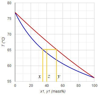
Calculating the vapor pressure for a given temperature is relatively easy according to section 4.2 (Raoult's-law). The solution of its reverse in case of a single material is also relatively simple (see: both the Antoine and the Clausius-Clapeyron equations can be inverted to express ecplicitly the T). But for a multicomponent system it is not trivial how to get the boiling temperature T of pmix.
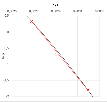
Literature recommends in general iterative methods, just like the quasi-Newton secant method, which have been used by early versions of VLE-Calc.com. Now, the App uses a method wich is based on the fact that the vapor pressure function of ln(p) − 1/T is quasi-linear (even in case of a multi-component system), altough not in a very wide temperature range. The algorithm:
- first we calcualte the boiling temparature of all of the pure components at the give pressure
- then we calculate the vapor pressure of the mixture at the lowest and at the highest temperature
- based on the 2-2 pressure-temperature data we now fit a linear function on ln(p) − 1/T (slope and intersect)
- based on the fitted linear function one could calculate the searched temperature for the given temperature - this is the bubble point of the mixture at the given pressure.
- For the third temperature we got, we calculate again the vapor pressure of the mixture. (This should be very close to the given pressure. If not, something were wrong along the calculations.)
- Now we may fit a cubic function (instead of a linear one) based on the calculated 3-3 ln(p) and 1/T values, and we get the bubble temperature of given pressure from this.
- (When vapor composition is necessary, the one should calculate one more time the mixture vapor pressure at the final bubble temperature, and the composition obtains as a by-product of the results.)
Note: this result is relatively accurate. Error is about 0.1░C. For less demanding applications one can stop at this point. But this result can be made much more accurate at relatively low cost, with several orders of magitude.
This method is computationally cheap (thus fast), mixture vapor pressure should be calculated only four-times in order to get the most accurate result, while the secant method usually needs more.
Introduction
Various liquid materials are either miscible, or not. (But that is certain.) Well, it is well-known that hydrocarbons and lots of other organic stuffs do not mix with water, but there are plenty of cases where it is not trivial at all whether the mixture splits to multiple liquid phases, or not.
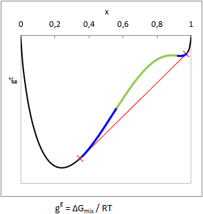
In principle, liquid phase split can be predicted from the curvature of the Gibbs free energy of mixing function (gE = ΔGmix.(x,T)/RT): when the function is convex from below at a composition range, i.e. ∂2gE(x,T)/∂x2 < 0, then the mixture will split to multiple liquid phases. This range is the unstable zone (see as green in the picture).
In case of two components the composition of the phases can be predicted by aligning a tangent line according to the figure (see as red line). In equilibrium the activity (ai=γi⋅xi) of all components are equal in all phases, so a computationally equivalent solution is to find the compositions with isoactivity (ai,phase-1 = ai,phase-2).
In practice, there is some trouble with this. One can notice in the figure that the gE function above the red tangent line is not everywhere convex from below (see as blue in the picture). This is the metastable zone. If the gross composition of a mixture falls into the metastable zone, testing the sign of the second derivate will not show that the mixture is biphasic.
In case of three or even more components the situation becomes more complicated, because the concepts (zones) described above should be interpreted and computationally handled on two or more dimensional surfaces. Practice of this is very not trivial, several article were published in this topic in the recent decades. Former versions of VLE - Calc .com used to use methods based on second derivate tests and isoactivity searches described above, thus the algorithms could not detect heterogenity in all cases. Another critical problem was that these algorithms produced sometimes erroneous equilibrium concentrations, the tie lines on the LLE-diagrams did not lined up consistently, even crossing tie-lines occurred. (The latter was not due to a bug in the program code, but due to properties of the thermodynamic model - see later in this chapter).
Liquid stability test
Due to the problems described in the introduction, the method of Wasylkievich et al were adopted to current version of VLE - Calc .com. This one is a very sophisticated approach that seemes to be reliable - though it was extremely difficult to reproduce and implement here.
The essence of the method is that the local minima (or inflexion points) of the so-called Tangent-Plane-Distance-Function (TPDF) have to be located, and the equilibral compositions of the liquid phases should be searched starting from the found local minima. The method has several advantage:
- indicates heterogenity even in the metastable zone
- can be used for any number of components (in theory)
- it provides very good starting points for finding the equilibrium compositions
- indicates when the found equilibral composition are false
- indicates when the system splits into more than 2 phases (in case of more than 2 components)
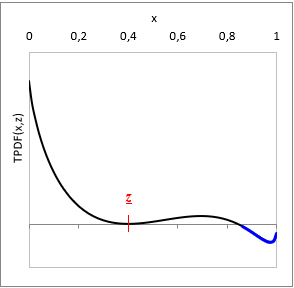
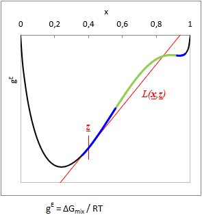
At a given T temperature and z gross mixture composition:
TPDF(x) = gE(x) − L(x, z)
where L(x, z) is a function tangent to gE at z gross mixture composition.
Is TPDF(x, z) negative in any x, then the liquid mixture is unstable, and will split to multiple phases. (See with blue on the TPDF figure)
Two-component systems
In case of a binary system the local minima of the TPDF (as well as inflexions and local maximum) can be found at the zeros of the 1st derivates. In current implementation these roots are searched by a quasi-Newton method. Not all roots will be searched, but the two probably closest to the minima of the TPDF.
In this method we exploit some useful properties of the binary gE function:
- there is no always local maximum, but if it exist, there is always only one.
- the slope of the function from the borders of the composition space into inward direction is always negative
Thus even if a local maximum exist, starting a search from the borders one would find always local minuma or inflexion point. The 1st derivate of the TPDF can be expressed by an approximate analytical derivative, and this expression should be made equal to zero:
∂TPDF(x1,2) / ∂x1 ≅ (ln x1 + ln γ1(x) − ln z1 − ln γ1(z)) − (ln x2 + ln γ2(x) − ln z2 − ln γ2(z)) = 0
The algorithm:
- Compute the activity coefficients at gross composition z, and store them (they are constants during the processγ1,2(z)).
- Start "guessed x"with point x1=0.
- Compute the activity coefficients at current x (γ1,2(x)).
-
Using the analytical derivate described above one can express the formulae below, from which the new x can be obtained:
c1 = ln γ1(x) − ln z1 − ln γ1(z)
c2 = ln γ2(x) − ln z2 − ln γ2(z)
x1,NEW = exp (−c1 + ln x2 + c2)
x2,NEW = 1 − x1,NEW
- Calculate the activity coefficients again with the new x value, and iterate the process until convergence. The resultant x is the closest minimum or inflexion to x1=0.
- Repeat the process described above starting from x1=1. From this process can be obtained the second local minimum or inflexion - if it exist. Namely, if there is only one minimum and no inflexion then both process gets to the same result, hence the system is homogenous.
Check the sign of the TPDF at the resultant x values. If it is negative, the system is unstable (heterogenous, biphasic). Now proceed searching for equilibral compositions of the phases, using these x values as starting points (this process is the "LLE-flash"). In general the Rachford-Rice equation is used for that (see below).
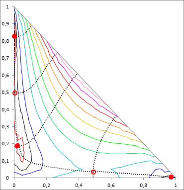
Systems with three or more components
As mentioned in the introduction, the situation in case of a multicomponent system is much more complicated as in binary case. The method of S. Wasylkievich et al handles the situation with high reliability, in case of any number of components. However the process is computationally quite intensive. I would not go into the formulas here anymore, everything is described in detail in the cited article.
The essence of the method is that in the case of n component the a TPDF is a (n−1)-dimensional surface, and the local minima of it has to be find. This surface is "crumpled cloth"-like, it has local minima (full red dots on the figure), local maximum can occur on it, and there can be saddle points (empty red dots on the figure). These points are called the stationary points of TPDF. In these points all the partial derivatives of the TPDF, by mole fractions of all i components, are zero ( ∂ TPDF(x) / ∂xi = 0). These stationary points are connected by "ridges" and "valleys", and according to the method, theese points are searched by tracking these ridges and valleys, along the whole (n−1)-dimensional composition space.
Once the minima are found, similarly to the binary case, the sign of TPDF at the minimums are checked, whether it is negative or positive. If any of the minima is negative, the system is unstable (heterogenous). Then proceed searching for the equilibral compositions of the phases, using the x values of the local minima as starting points (this process is the "LLE-flash"), and with solving the Rachford-Rice equation is used for that (see below).
Unfortunately, in multicomponent case, the first obtained phase compositions are not surely correct - it has to be checked. It can happen that not only one, but more isoactivity point-pairs can be found for a given z gross composition. From these solutions, the one with the lowest total Gibbs free energy of the system is correct.
So the obtained phase compositions have to be tested for stability, according to the ridge tracking technique described above (let z = xone-of-the-phases). If xone-of-the-phases is stable (i.e. no negative local minimum found), then the found equilibral phase compositions are correct. If the stability test results unstable (negative local minimum are found), then the found equilibral phase compositions are incorrect, and the LLE-flash process has to be repeated using the mole fractions of the local minima obtained in the last stability test, as initial values.
From the number of local minima, it can be assumed how many liquid phases are, but there is no guarantee that it is actually as much. E.g. if there are three minima, it is worth assuming this, and then look for three equilibrium phases based on the minima. If there were no three phases, it would be revealed either in the Rachford-Rice calculations (the system automatically reduces to 2-phase) or in the stability test of the found phase compositions.
The Rachford-Rice equation
Once it is known that the system is heterogenous, it is time to calculate the accurate composition of the coexisting luqid phases. In equilibrium the activity of the components (ai=γi⋅xi) is equal in all phases. At the same time it has to be also take into account that the material balance of each component must be in order, i.e. the total amount of each component in the separate phases must be equal to that of in the gross mixture (z). Rachford and Rice derived a very useful little equation for this task, solving it leads to results that meet both expectations at the same time:
- F(α) is the objective function, which has to be equal to zero
- α is a number between 0 and 1, which measures the molar amount of the 1st separate phase, from 1 mole gross mixture. (The molar amount of the 2nd phase is logically 1−α.)
- zi is the mole fraction of component i in the gross mixture
- Ki is the distribution ratio of component i: Ki = xi,phase 1/xi,phase 2 = γi,phase 2/γi,phase 1
The Rachford-Rice equation can be solved by iterative way:
- In the first step calculate the distribution ratios Ki using the assumed phase compositions and activity coefficients originating from the liquid stability test.
- Determine α by the Newton-Raphson method. Substitue everything into F(α) and into it's first derivate according to α, and the next approximation of α can be obtained by the formula: αnew = αprevious − F(αprevious) / F'(αprevious). Repeat with the new α and iterate until convergence.
- Calculate the phase compositions with the formulae:
xi,phase 1 = zi / (1 + α(Ki − 1))
xi,phase 2 = xi,phase 1 ⋅ Ki - Normalize the obtained mole fractions (for all phases): xi = xi / ∑nj=1 xj
- Calculate the activity coefficients using the new phase compositions, and calculate again all Ki, and iterate the whole process until convergence.
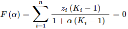
Boiling point / vapor pressure map by contour lines
Although it is not the most useful representation, but this type is the oldest triangle diagram in this app, since it is relatively simple and can be obtained quickly. Basically it represents the boiling point (bubble point, in isobaric case) or the vapor pressure (in isothermal case) of a ternary mixture, using contour lines. It's disadvantage is that the vapor composition (as additional information) does not appear in any form in this mode of representation.
At first, the triangular composition space is divided into many small triangles with a resolution of 20x20, and a VLE calculation is performed at each corner point of each small triangle. The minimum and maximum temperature or vapor pressure values are determined from all of the VLE results, and 8 values are selected between them, for the 8 contour lines. These are the "constant values", since these values are constant along the contour lines. With each constant value, all the small triangles are checked wether this value appears in it, or not. If a constant falls between the lowest and highest temperature/pressure values at the corners of the small triangle, then the contour line of the constant value passes through the given small triangle. If so, the position of the crossing section in the triangle is calculated by linear interpolation, and stored.
Plotting all of the crossing sections the contour lines outlined.
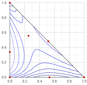
Residue curve map

For distillation problems, the residue curve is a much more useful representation than the boiling point map. The residue curve lies along the path as the composition of the bottom product changes during a batch distillation process. Logically, it moves from the more volatile regions to the less volatile regions, and the direction of the curve at each point is determined by the equilibrium x − y vector, characteristic of that point.
The shape of residue curve diagrams can be very diverse. In fact, the azeotropic points of a given ternary system, basically determine the shape of the figure. The azeotropic points (together with the corner points of the entire triangular diagram, which represent the pure components) divide the total composition space into smaller areas. Simple batch distillation processes can operate generally in these areas, in which the starting composition falls, so with the help of the residue curve set, it can be easily determined visually whether a given separation task is possible or not.
At first the azeotropic points of the system are located, then the corner points of the whole triangular diagram are added to the set. These points are called nodes. The set of nodes is arranged in triangles by Delaunay triangulation. Within each small triangle, residue curves are generated starting from one or more points.
During generation of a residue curve, the area of the small triangle is scanned from the starting point first in the x → y direction and then in the x ← y direction until a node is reached. Then another starting point is chosen and scan again.
Liquid miscibility phase-diagram
Liquid-liquid equilibrium diagrams have numerous types, these are not discussed here just the method of figure making.
At first the algorithm tests for liquid stability the binary subsystems representing the edges of the triangle diagram. The phase compositions of the miscibility gaps of the heterogenous binaries are stored for drawing on the one hand, on the other hand they are used for define starting points in the middle of the gaps.
Then it starts stepping from the starting points in small steps towards the inside of the triangle and determines the ternary tie-lines or conodes. The direction is determined by the slope of the tie-line (the direction is always perpendicular to the last tie-line), and the step size depends on the length of the tie-line - the shorter the tie-line, the smaller the step size. (These rules are basically for aesthetic purposes.)
If the algorithm finds a three-phase region, it continues to stepping from the middle of the other two edges of the triangle formed by the compositions of the three phases. Finally, plots all the found tie-lines.
In case of ternary vapor-liquid equilibrium calculations, the liquid-liquid equilibrium tie-lines are precalculated, stored, and arranged in small and thin triangles. Before starting the VLE calculation, the program checks if the given liquid composition falls into any of the LLE triangles. If so, it determines the composition of the separated liquid phases in a simplified procedure and performs VLE calculations with these compositions. (This precalculation and store-the-LLE-map mess is necessary because the liquid stability test is computationally very intensive. Less stability testing is required for an LLE diagram than for a batch distillation.)
During a single stage continuous distillation (flash distillation) process the starting liquid mixture (feed stream) is evaporated partially. The composition of the head- and bottom product depends on the evaporated proportion. In case of total evaporation (no bottom product) the composition of the distillate is the same as that of the starting mixture. In case of no evaporation (only bottom product), logically the bottom product is the same as the feed. The intermediate (real) situation is calculated using the Rachford-Rice equation (just like in case of liquid-liquid equilibrium).
where
- F(α) is the objective function, which has to be equal to zero
- α is the evaporated proportion, a number between 0 and 1, the molar amount of the vapor phase from 1 mol feed mixture. (The molar amount of the bottom product
- zi is the mole fraction of component i in the feed stream
- Ki is the distribution ratio of component i between the vapor and liquid phase: Ki = yi/xi
The Rachford-Rice equation can be solved by iterative way:
- The evaporated proportion α is given, constant.
- At first perform a bubble point calculation using the z feed composition.
- Calculate distribution ratios (as astarting approximation) using the resultant y values: Ki = yi/zi
- Calculate the composition of vapor and liquid phase:
xi = zi / (1 + α(Ki − 1))
yi = xi ⋅ Ki -
Normalize the mol fractions:
xi = xi / ∑nj=1 xj
yi = yi / ∑nj=1 yj - Perform another bubble point calculation using the resultant x values, and then recalculate the distribution ratios with the new y values (Ki = yi/xi), and iterate until convergence.
Batch distillation is a timely process, the composition of both the boiling liquid and the distillate changes over time. To model this, the process is divided into n equal parts. VLE-Calc.com always uses a resolution of n = 200, even if a lower resolution is given in the form, and only shows as much of the results in the table as specified. The program always performs the calculations in molar units.
The initial x composition of the mixture is given. The amount of the starting mixture is always n = 200 mol as described above (this made the code simpler), which is of course converted at the end according to the amount (and unit) specified by the user. A bubble point calculation is performed from x, and with the obtained vapor composition y one can calculate the amount of all components from the first evaporated dn = 1 mol:
nnew = nold − dn
xi,new = (xi,old ⋅ nold − yi ⋅ dn) / nnew
Store the new boiling liquid composition and calculate from this again the vapor composition, and so on, iterate until the liquid runs out completely.
Physico-chemical models operate usually with molar amounts and mole fractions, but in practice, man can usually think in mass and volume units.
For one type of task it is practical to measure the temperature in ░C, for another task in Kelvin.
It proven to be advantageous to build in an easy-to-use unit converter.
In this chapter one can study the converting methods and formulas.
Basic function
The unit converter module handles currently nine types of quantities, however, some of them has - for now - only 1 unit type built in. (I.e. it cannot be converted into another unit.) Every quantity type has a default unit, in which the numeric values are stored and the calculations are made with. When showing the numeric values on the page, the program calculates always from the default unit to the user selected unit.
The convertible quantity types and the selectable units are as follows:
| Quantity type | Default unit | Additional units |
| Molar weigth | g/mol | - |
| Liquid density | g/cm3 | - |
| Temperature | K (Kelvin) | ░C (Celsius), ░F (Fahrenheit) |
| Pressure | bar | kPa, atm, Hg mm, psi |
| Molar volume | cm3/mol | dm3/mol, m3/mol |
| Specific heat | kJ/kg⋅K | J/mol⋅K, kCal/kg⋅K, Cal/mol⋅K |
| Latent heat | kJ/mol | kJ/kg, kCal/mol, kCal/kg |
| Concentration or composition | mole fraction (x) | mass%, volume%, mol/dm3, g/100 cm3 |
| Quantity of material | kg | g, t, dm3, cm3, m3, mol, mmol, kmol |
Temperature conversion
| [K] | = | [░C] + 273.16 |
| [K] | = | ([░F] + 459.688) / 1.8 |
| [░C] | = | [K] − 273.16 |
| [░C] | = | ([░F] − 32) / 1.8 |
| [░F] | = | 1.8 ⋅ [K] − 459.688 |
| [░F] | = | 1.8 ⋅ [░C] + 32 |
Pressure conversion
| [bar] | [kPa] | [atm] | [Hg mm] | [psi] | ||
| [bar] | = | n.a | /100 | ⋅1.01325 | /750.0617 | /14.5037738007 |
| [kPa] | = | ⋅ 100 | n.a | ⋅101.325 | /7.500617 | /1450.37738007 |
| [atm] | = | /1.010325 | /101.325 | n.a | /760 | /14.6959488 |
| [Hg mm] | = | ⋅ 750.0617 | ⋅ 7.500617 | ⋅ 760 | n.a | ⋅ 51.71493367 |
| [psi] | = | ⋅ 14.5037738007 | ⋅ 0.145037738007 | ⋅ 14.6959488 | /51.71493367 | n.a |
Specific heat conversion
| [kJ/kg⋅K] | [J/mol⋅K] | [kCal/kg⋅K] | [Cal/mol⋅K] | ||
| [kJ/kg⋅K] | = | n.a | / M | / 4.1868 | /(4.1868⋅M) |
| [J/mol⋅K] | = | ⋅ M | n.a | ⋅ M /4.1868 | /4.1868 |
| [kCal/kg⋅K] | = | ⋅ 4.1868 | ⋅ 4.1868 / M | n.a | / M |
| [Cal/mol⋅K] | = | ⋅ 4.1868⋅M | ⋅ 4.1868 | ⋅ M | n.a |
where M is the mole weigth of the material.
Latent heat conversion
| [kJ/mol] | [kJ/kg] | [kCal/mol] | [kCal/kg] | ||
| [kJ/mol] | = | n.a | ⋅ 1000 ⋅ M | / 4.1868 | ⋅ 1000 ⋅ M / 4.1868 |
| [kJ/kg] | = | ⋅ 1000 / M | n.a | /(4.1868⋅M) | /4.1868 |
| [kCal/mol] | = | ⋅ 4.1868 | ⋅ 4.1868 ⋅ M | n.a | ⋅ M |
| [kCal/kg] | = | ⋅ 4.1868 / (1000⋅M) | ⋅ 4.1868 | / (1000⋅M) | n.a |
where M is the mole weigth of the material.
Concentration / composition conversion
Conversion between various concentration types is somewhat more difficult compared to the simpler ones above, because the calculations need some of the physical data of the components.
| [mole fraction] (x) | [mass%] (w) | [vol.%] (v) | [mol/dm3] (c) | [g/100 cm3] (ρ) | ||
| xi | = | n.a | wi Mi ⋅ ∑nj=1 (wj / Mj) |
vi⋅di Mi ⋅ ∑nj=1 (vj⋅dj / Mj) |
ci ∑nj=1 cj |
ρi Mi ⋅ ∑nj=1 (ρj / Mj) |
| wi | = | 100% ⋅ xi ⋅ Mi ∑nj=1 (xj ⋅ Mj) |
n.a | 100% ⋅ vi ⋅ di ∑nj=1 (vj ⋅ dj) |
100% ⋅ ci ⋅ Mi ∑nj=1 (cj ⋅ Mj) |
100% ⋅ ρi ∑nj=1 ρj |
| vi | = | xi⋅Mi di ⋅ ∑nj=1 (xj⋅Mj / dj) |
wi di ⋅ ∑nj=1 (wj / dj) |
n.a | ci⋅Mi di ⋅ ∑nj=1 (cj⋅Mj / dj) |
ρi di ⋅ ∑nj=1 (ρj / dj) |
| ci | = | 1000 ⋅ xi ∑nj=1 (xj ⋅ Mj / dj) |
1000 ⋅ wi Mi ⋅ ∑nj=1 (wj / dj) |
1000 ⋅ vi⋅di Mi ⋅ 100% |
n.a | 1000 ⋅ ρi Mi ⋅ 100 |
| ρi | = | 100 ⋅ xi ⋅ Mi ∑nj=1 (xj ⋅ Mj / dj) |
100 ⋅ wi ∑nj=1 (wj / dj) |
100 ⋅ vi ⋅ di 100% |
100 ⋅ ci ⋅ Mi 1000 |
n.a |
where M is the mole weigth, and di is the liquid density of component i.
Important notes: quantities per volume calculated using these formulas are not accurate, due to the so-called volume contraction phenomenon and to the temperature dependence of liquid density, which are not taken into account by these formulas. The order of magnitude of this inaccuracy may approx. a few rel.%.
New figures
The calculation methods of VLE-Calc.com allow to construct new useful diagrams, as well as to extend existing figures with additional information. Some of the plans:
- p-T phase diagram of multicomponent mixtures ("phase envelope")
- p-V phase diagram of multicomponent mixtures
- azeotropic composition in function of the pressure
- figure illustrating batch distillation processes (composition change of distillate or residue)
- ternary VLE-diagram extended with LLE-diagram drawn on it
New functions
Some upgrades for more convenient use and for usefulness in even more areas are also in the plans.
- mixtures with more than 3 components
- rectification (fractional distillation) calculation
- handling of distillate fractions (fore run, after run) at distillation calculation
- predicting physical properties of pure compounds using group contribution methods
- predicting physical properties of mixtures
- calculation of temperature-dependent physical properties at user-given temperature
- putting more and more new compounds into the database
- ability to handle custom (user-given) molecule
Known bugs and deficiencies
Onfortunatelly this new version of the app has some new bugs. Although, since the release of current version several errors have been found (thanks a lot for every feedback!), what could be fixed quickly was fixed quickly.
However, there is a stubborn, hidden bug - or malfunction - that could not be fixed yet. It occurs most often when dealing with ternary, heterogeneous systems; the program stops with an error message when attempting to do VLE calculations. The probability of this run-time error is higher, when very low concentrations are there among the LLE-data. The root cause of the malfunction has been largely determined, but no reassuring solution has been found so far.
Another annoying novelty is that the new LLE-procedure (the new liquid stability test) is computationally very intensive, thus slow even on todayÆs fast computers. (Although it is more reliable and knows more than the old one in return.) One of the goals is to change this as well.
Outlook
Several projects are in progress or are planned, which are more or less similar to VLE-Calc.com, but are to be used at different areas. An example of them is solubility.info which deals mainly with the solubility of solids in solvent mixtures. Another example may be azeotrope.info which moved recently to its own domain name.
An interesting and good news may be for those, who asked about a downloadable version of VLE-Calc.com (which does not exist), that an Excel version is under development. Most of the work is done already, product finalization, testing and debugging is in progress now. It is planned to publish in 2021.
Methods of calculations
-
A. Fredenslund, R.L. Jones, J.M. Prausnitz: Group-contribution estimation of activity coefficients in nonideal liquid mixtures, AIChE Journal, Vol. 21, No. 6, 1975, page 1086-1999
(DOI: 10.1002/aic.690210607)
-
J. Gmehling, J. Li, M. Schiller: Modified UNIFAC model. 2. Present parameter matrix and results for different thermodynamic properties, Ind. Eng. Chem. Res. 1993, 32, 178-193
(DOI: 10.1021/ie00013a024)
-
S. Horstmann, A. Jab│oniec, J. Krafczyk, K. Fischer, J. Gmehling: PSRK group contribution equation of state: comprehensive revision and extension IV, including critical constants and alfa-function parameters for 1000 components, Fluid Phase Equilibria 227 (2005) 157¢164
(DOI: 10.1016/0378-3812(91)85038-V)
-
Stanislaw K. Wasylkiewicz et al: Global Stability Analysis and calculation of LLE in multicomponent mixtures, Ind. Eng. Chem. Res. 1996, 35, 1395-1408
(DOI: 10.1021/ie950049r)
- J. Gmehling et al.: Vapor-Liquid Equilibrium Data Collection series, 1981 Dechema
Activity coefficient
Equation of state
Liquid stability and LLE calculation
Vapor-phase dimerization
Data of substances
- E.W. Flick: Industrial Solvents Handbook, 5th ed., 1998 William Andrew Publishing/Noyes
(eBook ISBN: 9780815518099)
- NIST Chemistry Webbook
- Wikipedia
- R. H. Perry, Don W. Green: Perry's Chemical Engineers' Handbook, 1999 McGraw-Hill Inc.
-
Jr. W. Acree, J. S. Chickos: Phase Transition Enthalpy Measurements of Organic and Organometallic Compounds. Sublimation, Vaporization and Fusion Enthalpies From 1880 to 2010, J. Phys. Chem. Ref. Data, Vol. 39, No. 4, 2010
(DOI: 10.1063/1.3309507)
- I. Mellan: Source Book of Industrial solvents, vol.II. (Halogenated hydrocarbons), Reinhold Publishing Corp., N.Y., 1957
- ChemSpider
- Sigma-Aldrich catalog
-
B. E. Poling, J. M. Prausnitz, J. P. O'Connell: The Properties of gases and liquids, 5th ed., McGraw-Hill, 2001
(DOI: 10.1021/ja0048634)
-
P. Martins, P. Sbaite, C. Benites, M. Maciel: Thermal Characterization of Orange, Lemongrass, and Basil Essential Oils; School of Chemical Engineering, University of Campinas (UNICAMP), 13083-970, Campinas ¢SP, Brazil
(DOI: 10.3303/CET1124078)
- PubChem
-
S. Horstmann, A. Jab│oniec, J. Krafczyk, K. Fischer, J. Gmehling: PSRK group contribution equation of state: comprehensive revision and extension IV, including critical constants and alfa-function parameters for 1000 components, Fluid Phase Equilibria 227 (2005) 157¢164
(DOI: 10.1016/0378-3812(91)85038-V)
-
N. N. Greenwood, A. Earnshaw: Chemistry of elements, Second edition, Butterworth-Heinemann, ® Reed Educational and Professional Publishing Ltd 1984, 1997
(eBook ISBN: 9780080501093)